
Abstract
This report will review what a metaball is, discuss the use of meta surface and object modelling, how it is implemented and applied to organic modelling, particles and fluid dynamics and liquid simulation in 3D modelling software, what types of meta surfaces/objects can be found and how to use/render them. It will also look at alternative methods, discussing the advantages and disadvantages of the various methods currently used within visual effects environment. Metaballs, are spheres which can influence one another to create an organic-looking, smooth surface in 3D modelling software using mathematic algorithms. Outlining a brief history of the development of the algorithms, without going into too much technical details, in this document. This paper will show what types of meta surfaces and object modelling are available, where they are used and how they are implemented in software.
Introduction
In three dimensional computer graphics 3D modelling is used to create a representation of a physical body, this is displayed as a two-dimensional image in either a computer simulation, rendered still images or animations. The typical method of modelling a surface in a computer graphic application is by defining points on the surface calculated by using parametric equations, these points are then connected to each other to form a mesh of polygons. This is the one of the best and quickest way to compute surface normals and perform transformations.
Fig 1: Parametric Equations
Implicit representation is an alternative to the parametric method way of calculating polygonal meshes. Implicit representations means that the surfaces are not explicitly calculated by the location of the vertices (like meshes are) or control points (like surfaces are), this is where a surface begins at a zero point and is contoured by the calculation of two or three variables. Mathematical equations are calculated on-the-fly by the software to create the meta object. The strengths of implicit representations are in operations such as blending and transformation, and have become one of the most popular methods used in special effects or as a base in modelling. You could use a collection of meta objects to form the primary shape of a model and then convert it to another object type for additional modelling. The rendering of Meta object is also very efficient.
Metaballs

 Metaballs, also known as blobby objects, are a type of implicit modelling technique (Ward. M, 2015). If we think of a metaball as a density field with a particle in its centre, where the particles density influence (how much affect it has on other objects) decreases the further away from the centre of the particle it travels. Taking an isosurface (defined by the X,Y,Z coordinates plus volume data) through this density field, a polygonal surfaces is created, this equates to a higher value of the isosurface, the closer it is to the particle. Metaball are extremely powerful because of the way they can be combined. Simply calculating the density field of each metaball to any given point, a very smooth fall off of the Blobby objects surface is achieved.
Fig 2: Combining of metaballs (Ward,M. (2015))
Jim Blinn invented the technique for rendering metaballs, he was a computer scientist and became well known when working for NASA as an expert in computer graphics, especially known for his work in animation in the voyager project and his research of the Blinn-Phong shading model, in the early 1980s. Blinn used exponentially decaying fields for each particle, with a Gaussian bump. To make this process more efficient the squared distance is used to avoid the more complicated process of computing the squared root. The density of any location is then calculated by summing all the isosurface values from all the particles. To create animation of DNA for Carl Sagan’s COSMOS TV Series, Jim Blinn proposed approximating each atom by a Gaussian potential, and using superposition of these potentials to define a surface. He ray traced these and called them “blobby models”. (Pugliese, M.1992)
Wyvill ET. Al. simplified the calculations by defining a cubic polynomial based on the radius of influence for a particle and the distance from the centre of the particle to the field location in question. (Ward. M, 2015) they called their creations “soft objects”. The Wyvill brothers ‘Soft Object’ model delivers a higher amount of smoothness and still avoids square roots.
Fig 3: Explaining the math Involved (Wong, J. 2014)
The Math
As a bit of a refresher, this is the equation of a circle centered at (x0,y0) with radius r:
(x−x0)2+(y−y0)2=r2
Or if you wanted to model all the points inside or on the boundary the circle, it would be this:
(x−x0)2+(y−y0)2≤r2
Rearranging this a little, we get this:
r2(x−x0)2+(y−y0)2≥1
When we have a bunch of circles bouncing around, we can model all the points inside of any of the circles like this, if circle i is defined by radius ri, and center (xi,yi):
maxi=0nr2i(x−xi)2+(y−yi)2≥1
The thing that makes metaballs all blobby-like is that instead of considering each circle separately, we take contributions from each circle. This models all of the points inside of all the metaballs:
∑i=0nr2i(x−xi)2+(y−yi)2≥1
We’re going to be using the left hand side of this inequality quite a bit, so let’s say:
f(x,y)=∑i=0nr2i(x−xi)2+(y−yi)2
If we sample the f(x,y) in a grid and plot the results, we get something like this:

The cells highlighted in green have a sample with f(x,y)>1 at their center.
If we increase the resolution, we start getting a kind of amoeba-blobby effect.

You might be thinking that this still looks a little blocky. We sampled in a grid, so why didn’t e just sample every pixel instead to make it look smoother? Well, for 40 bouncing circles, on a 700×500 grid, that would be on the order of 14 million operations. If we want to have a nice smooth 60fps animation, which would be 840 million operations per second. JavaScript engines may be fast nowadays, but not that fast.
A simple way to think of the metaball equation is to think that it is applying a falloff curve to ‘distance-from-lines’ or distance-from-curve’ then the ‘polygonization’ of the isosurface in render.
There are a many ways in which we can render the metaballs to display on screen. In the case of 3D metaballs, most commonly used are brute force ray-casting and the marching cubes algorithm.
The Marching Squares algorithm generates an approximation for a contour line of a two dimensional scalar field (Wong, J. 2014). This algorithm is very useful and most people have seen it used in drawing the contours on an ordnance survey map to show the height information and within games to draw tilesets textures. Marching squares produces the render information for two dimensional visuals in the three dimensional world we use a three dimensional version of the algorithm, Marching cubes, which is the same concept but with far more complex configurations to deal with. The algorithm goes through all the cubes in a 3D grid of data, for each cube it works out which triangles (in rendering) to create vertices has the potential of 256 possible configurations for a cube, but by using symmetry this is whittled down to only 15 different variations. Even so the calculation of each of these variables would soon mount up and be a slow process to go through all the cubes in a grid that a simple scene would produce. So the algorithm understands that a cube contains triangles of the isosurfaces, so could its neighbours. Its starts by searching firstly for a cube that contains triangles then only looks iteratively through the neighbouring eight cubes, to make sure to get all the components it trace a ray from each particles centre to look for intersections of the isosurface. To put it another way it will find an approximation value of all the points on a line (taken from the centre of the metaball) that have the same function.
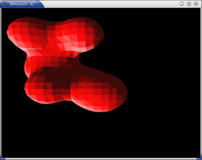
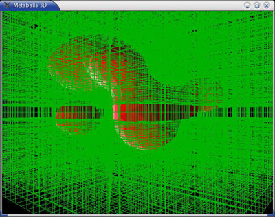
Fig 4: Marching Squares (Auclair,A. 2004)

Fig 5: 3D render using marching cubes – the 3d cube visualised in green (Auclair,A. 2004)
A rough example (but improving resolution all the time) is a MRI scan. You can think of these as slices of contours collated together to recreate a 3D object. The algorithm was developed by William Lorensen and Harvey Cline in the late 1980’s from the work they had been doing for General Electric to find a way to efficiently visualize data from MRI and CT scanning machines. The algorithm has been improved by many since then for example Evgeni V. Chernyaev’s Marching Cubes 33.
Types of Metas
There are five main types of metas, each one is influenced by its underlying structure.
- Meta Ball adds a meta with a point underlying structure.
- Meta Tube adds a meta with a line segment underlying structure.
- Meta Plane adds a meta with a planar underlying structure.
- Meta Ellipsoid adds a meta with an ellipsoidal underlying structure.
- Meta Cube adds a meta with a volumetric cubic underlying structure.
(Ardito, M. (2010) p463-469)
Each type of meta can be influenced by various controls within the 3D software.
Ball (point, zero-dimensional structure)
- This is the simplest meta, without any additional setting. As it is just a point, it generates an isotropic field, yielding a spherical surface (this is why it is called Meta Ball).
Tube (straight line, uni-dimensional structure)
- This is a meta which surface is generated by the field produced by a straight line of a given length. This gives a cylindrical surface, with rounded closed ends. It has one additional parameter:
dx: The length of the line (and hence of the tube – defaults to 1.0).
Plane (rectangular plane, bi-dimensional structure)
- This is a meta which surface is generated by the field produced by a rectangular plane. This gives a parallelepipedal surface, with a fixed thickness, and rounded borders. It has two additional parameters:
dx: The length of the rectangle (defaults to 1.0).
dy: The width of the rectangle (defaults to 1.0).
Note that by default, the plane is a square.
Elipsoid (ellipsoidal volume, tri-dimensional structure)
- This is a meta which surface is generated by the field produced by an ellipsoidal volume. This gives an ellipsoidal surface. It has three additional parameters:
dx: The length of the ellipsoid (defaults to 1.0).
dy: The width of the ellipsoid (defaults to 1.0).
dz: The height of the ellipsoid (defaults to 1.0).
Note that by default, the volume is a sphere, producing a spherical meta, as the Ball option)
Cube (parallelepipedal volume, tri-dimensional structure)
- This is a meta which surface is generated by the field produced by a parallelepipedal volume. This gives a parallelepipedal surface, with rounded edges. As you might have guessed, it has three additional parameters:
dx: The length of the parallelepiped (defaults to 1.0).
dy: The width of the parallelepiped (defaults to 1.0).
dz: The height of the parallelepiped (defaults to 1.0).
Note that by default, the volume is a cube.
(Ardito, M. (2010) p463-469)
The influence of each meta surface/object can be adjusted by manipulating the threshold of the field emitted. This setting is usually a global setting, meaning it will make a uniformed adjustment to all the objects (particles) in the group allow them to interact with each adjacent objects therefore giving them the blobby object look. There are two attributes that can be altered, positive and negative. A positive threshold will work as an attraction to other meta surfaces around it, the negative will repel other meta surfaces, the amount of influence will vary dependant on the distance of the surface from each other.
Examples
Positive.
A positive influence is defined as an attraction meaning the meshes will stretch towards each other as the rings of influence intersect. (Positive) shows two meta balls’ ring of influence intersecting with a positive influence.

Notice how the meshes have pulled towards one another. The area circled in white shows the green influence rings intersecting.
Negative.
The opposite effect of a positive influence would be a negative influence: the objects repel each other. (Negative) shows a meta ball and meta plane where the first is negative and the second, positive. Notice how the negative meta is not visible: only the surrounding circles appear. This is how Blender indicates that the object is negative.

The white arrow indicates how the sphere is repelling or pushing away the plane’s mesh. This causes the plane’s mesh to “cave in” or collapse inward. If you move the plane away from the sphere, the plane’s mesh will restore itself.
(Ardito, M. (2010) p463-469)
Discussion
Here are the positive and negatives of using Metaballs and a few alternatives stating what makes them more attractive
- Metaballs are spheres which can influence one another to create an organic-looking, smooth surface. These meshes often show thick borders and require a certain amount of filtering or correspondingly high particle counts to achieve a satisfying quality.
- Weighted isotropic is the best compromise between creation time and quality. This mode yields smooth meshes with slightly rounded borders. Filters can help to achieve a very good, realistic mesh.
- Weighted anisotropic creates meshes with thin borders, but sometimes the fluid has a torn look. To compensate for this effect, the → “Radius” parameter of the attached emitter’s “Field” panel should be increased.
- Mpolygons does not create a closed surface, but attaches a 2D polygon to every particles instead.
- Clone object attaches an object to every particle.
Nextbase (2015)
Conclusion
This report has covered what are meta surfaces/objects, how they are created and implemented, a little history on them, what types of meta object are available within 3D software and the positives/negatives of meta objects and their alternatives.
Meta surface objects are used widely throughout computer graphics, modelling and animation. They are especially useful at creating renders of fluid simulation due to the ability to attract or repel each other through their density fields therefore giving the simulation the impression of realism. Rendering the polygons created by the meta objects are power intensive but will give excellent results.
Most 3D (and some non-3D) software has options to create Meta objects within them. While carry out the research for this report a few names of the main application have reoccurred they are:
- Autodesk 3Ds Max and Maya (has quite advanced features for the creation of meta surfaces)
- Blender (also has well evolved features)
- Nextbase Realflow (the professional standard in creating fluids and soft body effects using metaballs and able to implement a couple alternatives)
This only scratches the surface of where meta objects are implemented and many other applications and implementations of these dynamic models are being used and newer, better method are invented all the time. It’s a fascinating and exciting area of the three dimensional graphic world.
References
Adrien, A. (2004) Metaballs 3d. [ONLINE] Available at: http://eldeann7.chez-alice.fr/meta3D/indexen.htm. [Accessed 23 October 15].
Ardito, M. (2010) Blender Wiki PDF Manual. Blender Manual 2.4, [Online]. 20100622, 462 -469. Available at: http://pdf.letworyinteractive.com/download/category/1-pdf [Accessed 28 October 2015].
Chaos Group. (2015) V-Ray 3.0 for Maya Help. [ONLINE] Available at:http://docs.chaosgroup.com/display/VRAY3MAYA/VRayMetaball. [Accessed 31 October 15].
Wyvill, G. McPhetters, C. Wyvill, B. (1986) Data Structure for Soft Objects, The Visual Computer, Vol. 2pp. 227-234
Goulekas, K, (2001) Visual Effects in A Digital World. San Diago: Morgan Kaufmann.
Blinn, J. (1982) A Generalization of Algebraic Surface Drawing, ACM Transactions on Graphics, Vol. 1, No. 3, pp. 235-256
Menon, J. (1996) An Introduction to Implicit Techniques, SIGGRAPH Course Notes on Implicit Surfaces for Geometric Modelling and Computer Graphics
Nextbase (2015) RealFlow Documentation. [ONLINE] Available at: http://support.nextlimit.com/display/rf2015docs/PL+-+Mesh. [Accessed 31 October 15].
Owen, S. (1999) Metaballs. [ONLINE] Available at: http://www.siggraph.org/education/materials/HyperGraph/modeling/metaballs/metaballs.htm. [Accessed 31 October 15].
Pugliese, M. (1992) A BRIEF HISTORY OF BLOBBY MODELING. [ONLINE] Available at: http://steve.hollasch.net/cgindex/misc/metaballs.html. [Accessed 14 October 15].
Ward,M. (2015) An Overview of Metaballs/Blobby Objects. [ONLINE] Available at: http://web.cs.wpi.edu/~matt/courses/cs563/talks/metaballs.html. [Accessed 14 October 15].
Wong,J. (2014) Metaballs and Marching Squares. [ONLINE] Available at: http://steve.hollasch.net/cginhttp://jamie-wong.com/2014/08/19/metaballs-and-marching-squares/dex/misc/metaballs.html. [Accessed 23 October 15].
Images
Figure 1: parametric equations, [ONLINE] Available at: http://web.mit.edu/hyperbook/Patrikalakis-Maekawa-Cho/node27.html (Accessed on 14 October15)
Fig 2: Combining of metaballs, Ward,M. (2015) An Overview of Metaballs/Blobby Objects. [ONLINE] Available at: http://web.cs.wpi.edu/~matt/courses/cs563/talks/metaballs.html. [Accessed 14 October 15].
Fig 4 and 5: Matching Squares, Adrien, A. (2004) METABALLS 3D. [ONLINE] Available at: http://eldeann7.chez-alice.fr/meta3D/indexen.htm. [Accessed 23 October 15].